So. Gaussian processes, eh.
Now that we know what they are, I guess we should do something with a Gaussian process. But we immediately hit a problem. You see, Gaussian processes are charming things, sweet and caring. But they have a dark side. Used naively1, they’re computationally expensive when you’ve got a lot of data.
Stab of dramatic music
Yeah. So. What’s the problem here? Well, the first problem is people seem to really like having a lot of data. Fuck knows why. Most of it is rubbish2. But they do.
This is a problem for our poor little Gaussian processes because of how the data tends to come.
A fairly robust model for data is that it comes like \[ (y_i, s_i, x_i), \] where \(y_i\) is our measurement of choice (which might be a continuous, discrete or weird3), \(s_i\) is our location4 in the index set5 \(\Omega\) (usually \(\Omega \subset \mathbb{R}^d\)) of the Gaussian process, and \(x_i\) is whatever other information we have6. If we want to be really saucy, we could also assume these things are iid samples from some unknown distribution and then pretend like that isn’t a wildly strong structural assumption. But I’m not like that. I’ll assume the joint distribution of the samples is exchangeable7 8 9. Or something. I’m writing this sequentially, so I have no idea where this is going to end up.
So where is the problem? The problem is that, if we use the most immediately computational definition of a Gaussian process, then we need to build \[ \begin{pmatrix} u(s_1)\\ u(s_2) \\ \vdots \\ u(s_n)\end{pmatrix} \sim N\left( \begin{pmatrix} \mu(s_1)\\ \mu(s_2) \\ \vdots \\ \mu(s_n)\end{pmatrix}, \begin{pmatrix} c(s_1, s_1) & c(s_1, s_2) & \cdots & c(s_1, s_n) \\ c(s_2, s_1) & c(s_2, s_2) & \cdots & c(s_2, s_n) \\\vdots &\vdots &\ddots &\vdots \\ c(s_n, s_1) & c(s_n, s_2) & \cdots & c(s_n, s_n)\end{pmatrix}\right). \] Where \(s_1,\ldots, s_n\) are all of the distinct values of \(s_i\) in the dataset. If there are a lot of these, the covariance matrix is very large and this becomes a problem. First, we must construct it. Then we must solve it. Then we must do actual computations with it. The storage scales quadratically in \(n\). The computation scales cubically in \(n\). This is too much storage and too much computation if the data set has a lot of distinct GP evaluations, it will simply be too expensive to do the matrix work that we need to do in order to make this run.
So we need to do something else.
A tangent; or Can we just be smarter?
On a tangent, because straight lines are for poor souls who don’t know about Gaussian processes, there’s a body of work on trying to circumvent this problem by being good at maths. The idea is to try to find some cases where we don’t need to explicitly form the covariance matrix in order to do all of the calculations. There’s a somewhat under-cooked10 literature on this. It dances around an idea that traces back to fast multipole methods for integral equations: We know that correlations decay as points get further apart, so we do not need to calculate the correlations between points that are far apart as well as we need to calculate the correlations between points that are close together. For a fixed covariance kernel that decays in a certain way, you can modify the fast multipole method, however it’s more fruitful to use an algebraic11 method. H-matrices was the first real version of this, and there’s a paper from 2008 using them to approximate GPs. A solid chunk of time later, there have been two good papers recently on this stuff. Paper 1 Paper 2. These methods really only provide gradient descent type methods for maximum likelihood estimation and it’s not clear to me that you’d be able to extend these ideas easily to a Bayesian setting (particularly when you need to infer some parameters in the covariance function)12.
I think this sort of stuff is cool for a variety of reasons, but I also don’t think it’s the entire solution. (There was also a 2019 NeurIPS paper that scales a GP fit to a million observations as if that’s a good idea. It is technically impressive, however.) But I think the main possibility of the H-matrix work is that it allows us to focus on the modelling and not have to make premature trade offs with the computation.
The problem with modelling a large dataset using a GP is that GPs are usually fit with a bunch of structural assumptions (like stationarity and isotropy) that are great simplifying assumptions for moderate data sizes but emphatically do not capture the complex dependency structures when there is a large amount of data. As you get more data, your model should become correspondingly more complex13 and stationary, and/or isotropic Gaussian processes emphatically do not do this.
This isn’t to say that you shouldn’t use GPs on a large data set (I am very much on record as thinking you should), but that it needs to be a part of your modelling arsenal and probably not the whole thing. The real glory of GPs is that they are a flexible enough structure to play well with other modelling techniques. Even if you end up modelling a large data set with a single GP, that GP will most likely be anisotropic, non-stationary, and built up from multiple scales. Which is a different way to say that it likely does not have a squared exponential kernel with different length scales for each feature.
(It’s probably worth making the disclaimer at this point, but when I’m thinking about GPs, I’m typically thinking about them in 1-4 dimensions. My background is in spatial statistics, so that makes sense. Some of my reasoning doesn’t apply in more typical machine learning applications where \(s_i\) might be quite high-dimensional. That said, you simply get a different end of the same problem. In that case you need to balance the smoothness needed to interpolate in high dimensions with the structure needed to allow your variables to be a) scaled differently and b) correlated. Life is pain either way.)
So can we make things better?
The problem with Gaussian processes, at least from a computational point of view, is that they’re just too damn complicated. Because they are supported on some infinite dimensional Banach space \(B\), the more we need to see of them (for instance because we have a lot of unique \(s_i\)s) the more computational power they require. So the obvious solution is to somehow make Gaussian processes less complex.
This somehow has occupied a lot of people’s time over the last 20 years and there are many many many many possible options. But for the moment, I just want to focus on one of the generic classes of solutions: You can make Gaussian processes less computationally taxing by making them less expressive.
Or to put it another way, if you choose an \(m\) dimensional subspace \(V_m \subset B\) and rep;ace the GP \(u\), which is supported on the whole of \(B\), with a different Gaussian process \(u_m\) supported on \(V_m\), then all of your problems go away.
Why? Well because the Gaussian process on \(V_m\) can be represented in terms of an \(m\)-dimensional Gaussian random vector. Just take \(\phi_j\), \(j=1,\ldots, m\) to be a basis for \(V_m\), then the GP \(u_m\) can be written as \[ u_m = \sum_{j=1}^m w_j \phi_j, \] where \(w \sim N(\mu, \Sigma)\), for some \(\mu\) and \(\Sigma\). (The critical thing here is that the \(\phi_j\) are functions so \(u_m\) is still a random function! That link between the multivariate Gaussian \(w\) and the function \(u_m\) that can be evaluated at any \(s_i\) is really important!)
This means that I can express my Gaussian process prior in terms of the multivariate Gaussian prior on \(w\), and I only need \(\mathcal{O}(m^3)\) operations to evaluate its log-density.
If our observation model is such that \(p(y_i \mid u) = p(y_i \mid u(s_i))\), and we assume conditional14 independence, then we can eval the log-likelihood term \[ \sum_{i=1}^n p(y \mid u_m(s_i)) = \sum_{i=1}^n p(y \mid a_i^Tw) \] in \(\mathcal{O}(m^2 n)\) operations. Here \([a_i]_j = \phi_j(s_i)\) is the vector that links the basis in \(u_n\) that we use to define \(w\) to the observation locations15.
Many have been tempted to look at the previous paragraph and conclude that a single evaluation of the log-posterior (or its gradient) will be \(\mathcal{O}(n)\), as if that \(m^2\) multiplier were just a piece of fluff to be flicked away into oblivion.
This is, of course, sparkly bullshit.
The subspace size \(m\) controls the trade off between bias and computational cost and, if we want that bias to be reasonably small, we need \(m\) to be quite large. In a lot of cases, it needs to grow with \(n\). A nice paper by David Burt, Carl Rasmussen, and Mark van der Wilk suggests that \(m(n)\) needs to depend on the covariance function16. In the best case (when you assume your function is so spectacularly smooth that a squared-exponential covariance function is ok), you need something like \(m = \mathcal{O}(\log(n)^d)\), while if you’re willing to make a more reasonable assumption that your function has \(\nu\) continuous17 derivatives, then you need something like \(m = \mathcal{O}(n^\frac{2d}{2\nu-d})\).
You might look at those two options for \(m\) and say to yourself “well shit. I’m gonna use a squared exponential from now on”. But it is never as simple as that. You see, if you assume a function is so smooth it is analytic18, then you’re assuming that it lacks the derring-do to be particularly interesting between its observed values19. This translates to relatively narrow uncertainty bands. Whereas a function with \(\nu\) derivatives has more freedom to move around the smaller \(\nu\) is. This naturally results in wider uncertainty bands.
I think20 in every paper I’ve seen that compares a squared exponential covariance function to a Matérn-type covariance function (aka the ones that let you have \(\nu\)-times differentiable sample paths), the Matérn family has performed better (in my mind this is also in terms of squared error, but it’s definitely the case when you’re also evaluating the uncertainty of the prediction intervals). So I guess the lesson is that cheap isn’t always good?
Anyway. The point of all of this is that if we can somehow restrict our considerations to an \(m\)-dimensional subspace of \(B\), then we can get some decent (if not perfect) computational savings.
But what are the costs?
Some notation that rapidly degenerates into a story that’s probably not interesting
So I guess the key question we need to answer before we commit to any particular approximation of our Gaussian process is what does it cost? That is, how does the approximation affect the posterior distribution?
To quantify this, we need a way to describe the posterior of a Gaussian process in general. As happens so often when dealing with Gaussian processes, shit is about to get wild.
A real challenge with working with Gaussian processes theoretically is that they are objects that naturally live on some (separable21) Banach space \(B\). One of the consequences of this is that we cannot just write the density of \(u\) as \[ p(u) \propto \exp\left(-\frac{1}{2}C_u(u, u)\right) \] because there is no measure22 on \(B\) such that \[ \Pr(u \in A) = \int_A p(u)\,du. \]
This means that we can’t just work with densities to do all of our Bayesian stuff. We need to work with posterior probabilities properly.
Ugh. Measures.
So let’s do this. We are going to need a prior probability associated with the Gaussian process \(u\), which we will write as \[ \mu_0(A) = \Pr(u \in A), \] where \(A\) is a nice23 set in \(B\). We can then use this as a base for our posterior, which we define as \[ \mu^y(A) = \Pr(u \in A \mid y) = \frac{1}{Z}\mathrm{e}^{-\Phi(u;y)}, \] where \(\Phi(u;y)\) is the negative log-likelihood function. Here \(Z\) is the normalising constant \[ Z = \mathbb{E}_\mu\left( \mathrm{e}^{-\Phi(u;y)}\right), \] which is finite as long as \(\exp(-\Phi(u;y)) \leq C(\epsilon)\exp(\epsilon\|u\|^2)\) for all \(\epsilon > 0\), where \(C(\epsilon)\geq 0\) is a constant. This is a very light condition.
This way of looking at posteriors resulting Gaussian process priors was popularised in the inverse problems literature24. It very much comes from a numerical analysis lens: the work is framed as here is an object, how do we approximate it?.
These questions are different to the traditional ones answered by a theoretical statistics papers, which are almost always riffs on “what happens in asymptopia?”.
I came across this work for two reasons: one is because I have been low-key fascinated by Gaussian measures ever since I saw a talk about them during my PhD; and secondly my PhD was in numerical analysis, so I was reading the journals when these papers came out.
That’s not why I explored these questions, though. That is a longer story. The tl;dr is
I had to learn this so I could show a particular point process model converges, and so now the whole rest of this blog post is contained in a technical appendix that no one has ever read in this paper.
Here comes the anecdote. Just skip to the next bit. I know you’re like “but Daniel just delete the bullshit text” but that is clearly not how this works.
Expand at your peril
I know these papers pretty much backwards for the usual academic reason: out of absolute spite. One of my postdocs involved developing some approximation methods for Markovian Gaussian processes25, which allowed for fast computation, especially when combined with INLA26, which is a fabulous method for approximating posterior distributions when a big chunk of the unobserved parameters have a joint Gaussian prior27.
One of the things that INLA was already pretty good at doing was fitting log-Gaussian Cox processes (LGCP), which are a type of model for point patterns28 that can be approximated over a regular grid by a Poisson regression with a log-mean given by (covariates +) a Gaussian process defined on the grid. If that process is Markov, you can get full posterior inference quickly and accurately using INLA. This compared very favourably with pre-INLA methods, which gave you full posterior inference laboriously using a truncated gradient MALA scheme in about the same amount of time it would take the US to get a high-speed rail system.
Anyway. I was in Trondheim working on INLA and the, at that stage, very new SPDE29 stuff (the 2011 JRSSSB read paper had not been written yet, let alone been read). Janine Illian, who is a very excellent statistician and an all round fabulous person, had been working on the grided LGCP stuff in INLA and came to Trondheim to work with Håvard30 and she happened to give a seminar on using these new LGCP methods to do species distribution mapping. I was strongly encouraged to work with Janine to extend her grid methods to the new shiny SPDE methods, which did not need a grid.
Janine had to tell me what a Poisson distribution was.
Anyway. A little while later31 we had a method that worked and we32 wrote it up. We submitted it to Series B and they desk rejected it. We then, for obscure reasons33, submitted it to Biometrika. Due to the glory of arXiv, I can link to the original version.
Although it was completely unlike anything else that Biometrika publishes, we got some quite nice reviews and either major revisions or a revise and resubmit. But one of the reviewer comments pissed me off: they said that we hadn’t demonstrated that our method converges. Now, I was young at the time and new to the field and kinda shocked by all of the shonky numerics that was all over statistics at the time. So this comment34 pissed me off. More than that, though, I was fragile and I hated the comment because I was new to this and had absolutely no fucking idea how to prove this method would converge. Rasmus Waagepetersen had proven convergence of the grid approximation but a) I didn’t understand the proof and b) our situation was so far away there was no chance of piggybacking off it.
It was also very hard to use other existing statistics literature, because, far from being an iid situation, the negative log-likelihood for a Poisson process35 on an observation window \(\Omega\) is \[ \Phi(u;y) = \int_\Omega e^{u(s)}\,ds - \sum_{s_i \in y}e^{u(s_i)} - |\Omega|, \] where the point pattern \(y\) is a (random) collection of points \(s_j\) and \(|\Omega|\) is the area/volume of the observation window. This is fundamentally not like a standard GP regression.
So, long story short36, I was very insecure and rather than admit that it was difficult to show that these approximations converged, I worked on and off for like 2 years trying to work out how to do this37 and eventually came up with a fairly full convergence theory for posteriors derived from approximate likelihoods and finite dimensional approximations to Gaussian processes38. Which I then put into the appendix of a paper that was essentially about something completely different.
I don’t have all that many professional regrets (which is surprising because I’ve made a lot of questionable choices), but I do regret not just making that appendix its own paper. Because it was really good work.
But anyway, I took the inverse problems39 work of Andrew Stuart and Masoumeh Dashti and extended it out to meet my needs. And to that end, I’m going to bring out a small corner of that appendix because it tells us what happens to a posterior when we replace a Gaussian process by a finite dimensional approximation.
How do we measure if a posterior approximation is good?
Part of the struggle when you’re working with Gaussian processes as actual objects rather than as a way to generate a single finite-dimensional Gaussian distribution that you use for analysis is that, to quote Cosma Shalizi40, “the topology of such spaces is somewhat odd, and irritatingly abrupt”. Or to put it less mathematically, it is hard to quantify which Gaussian processes are close together.
We actually saw this in the last blog where we noted that the distribution of \(v = cu\) has no common support with the distribution of \(u\) if \(|c| \neq 1\). This means, for instance, that the total variation between \(u\) and \(v\) is 2 (which is it’s largest possible value) even if \(c = 1 + \epsilon\) for some tiny \(\epsilon\).
More generally, if you’re allowed to choose what you mean by “these distributions are close” you can get a whole range of theoretical results for the posteriors of infinite dimensional parameters, ranging from this will never work and Bayes in bullshit to everything is wonderful and you never have to worry.
So this is not a neutral choice.
In the absence of a neutral choice, we should try to make a meaningful one! An ok option for that is to try to find functions \(G(u)\) that we may be interested in. Classically, we would choose \(G\) to be bounded (weak41 convergence / convergence in distribution) or bounded Lipschitz42. This is good but it precludes things like means and variances, which we would quite like to converge!
The nice thing about everything being based off a Gaussian process is that we know43 that there is some \(\epsilon > 0\) (which may be very small) such that \[ \mathbb{E}_{\mu_0}\left(\mathrm{e}^{\epsilon \|u\|_B^2}\right) < \infty. \] This suggests that as long as the likelihood isn’t too evil, the posterior will also have a whole arseload of moments.
This is great because it suggests that we can be more ambitious than just looking at bounded Lipschitz functions. It turns out that we can consider convergence over the class of functionals \(G\) such that \[ |G(u) - G(v)| \leq L(u) \|u - v\|_B, \] where \(\mathbb{E}_{\mu_0}(L(u)) < \infty\). Critically this includes functions like moments of \(\|u\|_B\) and, assuming all of the functions in \(B\) are continuous, moments of \(u(s)\). These are the functions we tend to care about!
Convergence of finite dimensional Gaussian processes
In order to discuss the convergence of finite dimensional Gaussian processes, we need to define them and, in particular, we need to link them to some Gaussian process on \(B\) that they are approximating.
Let \(u\) be a Gaussian process supported on a Banach space \(B\). We define a finite dimensional Gaussian process to be a Gaussian process supported on some space \(V_m \subset B\) that satisfies \[ u_n = R_m u, \] where \(R_m: B \rightarrow V_m\) is some operator. (For this to be practical we want this to be a family of operators indexed by \(m\).)
It will turn out that how this restriction is made is important. In particular, we are going to need to see how stable this restriction is. This can be quantified by examining \[ \sup_{\|f\|_V = 1} \|R_m f\|_{B} \leq A_m \|f\|_V, \] where \(A_m > 0\) is a constant that could vary with \(m\) and \(V \subseteq B\) is some space we will talk about later. (Confusingly, I have set up the notation so that it’s not necessarily true that \(V_m \subset V\). Don’t hate me because I’m pretty, hate me because I do stupid shit like that.)
Example 1: An orthogonal truncation
There is a prototypical example of \(R_m\). Every Gaussian process on a separable Banach space admits a Karhunen-Loève representation \[ u = \sum_{k = 0}^\infty \lambda_k^{1/2} z_k \phi_k, \] \(z_k\) are iid standard normal random variables and \((\lambda_k, \phi_k)\) are the eigenpairs44 of the covariance operator \(C_u\). The natural restriction operator is then \[ R_m f = \sum_{j=0}^m \langle f, \phi_j\rangle_{L^2}\phi_j. \] This was the case considered by Dashti and Stuart in their 2011 paper. Although it’s prototypical, we typically do not work with the Karhunen-Loève basis directly, as it tends to commit us to a domain \(\Omega\). (Also because we almost45 never know what the \(\phi_j\) are.)
Because this truncation is an orthogonal projection, it follows that we have the stability bound with \(A_m = 1\) for all \(m\).
Example 2: Subset of regressors
Maybe a more interesting example is the subset of regressors46. In this case, there are a set of inducing points \(s_1, \ldots, s_m\) and \[ R_m f = \sum_{j=1}^m w_j r_u(\cdot, s_j), \] where the weights solve \[ K_m w = b, \] \([K_m]_{ij} = r_u(s_i, s_j)\) and \(b_j = f(s_j)\).
It’s a bit harder to get the stability result in this case. But if we let \(V_m\) have the RKHS47 norm, then \[\begin{align*} \|R_m f\|^2_{H_u} &= w^TK_m w \\ &= b^T K^{-1} b \\ &\leq \|K^{-1}\|_2 \|b\|_2^2 \end{align*}\]
Assuming that \(B\) contains continuous functions, then \(\|b\|_2 \leq C\sqrt{m} \|f\|_B\). I’m pretty lazy so I’m choosing not to give a shit about that \(\sqrt{m}\) but I doubt it’s unimprovable48. To be honest, I haven’t thought deeply about these bounds, I am doing them live, on my couch, after a couple of red wines. If you want a good complexity analysis of subset of regressors, google.
More interestingly, \(\|K_m^{-1}\|_2\) can be bounded, under mild conditions on the locations of the \(s_j\) by the \(m\)-th largest eigenvalue of the operator \(Kf = \int_\Omega r_u(s,t)f(t)\,dt\). This eigenvalue is controlled by how differentiable \(u\) is, and is roughly \(\mathcal{O}\left(m^{-\alpha - d/2}\right)\) if \(u\) has a version with \(\alpha\)-almost sure (Hölder) derivatives. In the (common) case where \(u\) is analytic (eg if you used the squared exponential covariance function), then this bound increases exponentially (or squared exponentially for the squared exponential) in \(m\).
This means that the stability constant \(A_m \geq \|K_m^{-1}\|\) will increase with \(m\), sometimes quite alarmingly. Wing argues that it is always at least \(\mathcal{O}(m^2)\). Wathan and Zhu have a good discussion for the one-dimensional case and a lot of references to the more general situation.
Example 3: The SPDE method
My personal favourite way to approximate Gaussian processes works when they are Markovian. The Markov property, in general, says that if, for every49 set of disjoint open domains \(S_1\) and \(S_2 = \Omega \backslash \bar S_1\) such that \(S_1 \cup \Gamma \cup S_2\), where \(\Gamma\) is the boundary between \(S_1\) and \(S_2\), then \[ \Pr(A_1 \cup A_2 \mid B_\epsilon) = \Pr(A_1 \mid B_\epsilon) \Pr(A_2 \mid B_\epsilon), \] where \(A_j \in \sigma\left(\{u(s), s \in S_j\}\right)\) and50 \(B_\epsilon \in \sigma\left(\{u(s); d(s, \Gamma) < \epsilon\}\right)\) and \(\epsilon>0\).
Which is to say that it’s the normal Markov property, but you may need to fatten out the boundary between disjoint domains infinitesimally for it to work.
In this case, we51 know that the reproducing kernel Hilbert space has the property that the inner product is local. That means that if \(f\) and \(g\) are in \(H_u\) and have disjoint support52 then \[ \langle f, g\rangle_{H_u} = 0, \] which, if you squint, implies that the precision operator \(\mathcal{Q}\) is a differential operator. (That the RKHS inner product being local basically defines the Markov property.)
We are going to consider a special case53, where \(u\) solves the partial differential equation \[ L u = W, \] where \(L\) is some differential operator and \(W\) is white noise54.
We make sense of this equation by saying a Gaussian process \(u\) solves it if \[ \int_\Omega \left(L^*\phi(s)\right)\left( u(s)\right)\,ds \sim N\left(0, \int_\Omega \phi^2(s)\,ds\right), \] for every smooth function \(\phi\), where \(L^*\) is the adjoint of \(L\) (we need to do this because, in general, the derivatives of \(u\) could be a bit funky).
If we are willing to believe this exists (it does—it’s a linear filter of white noise, electrical engineers would die if it didn’t) then \(u\) is a Gaussian process with zero mean and covariance operator \[ \mathcal{C} = (L^*L)^{-1}, \] where \(L^*\) is the adjoint of \(L\).
This all seems like an awful lot of work, but it’s the basis of one of the more powerful methods for approximating Gaussian processes on low-dimensional spaces (or low-dimensional manifolds). In particular in 1-3 dimensions55 or in (1-3)+1 dimensions56 (as in space-time), Gaussian processes that are built this way can be extremely efficient.
This representation was probably first found by Peter Whittle and Finn Lindgren, Johan Lindström and Håvard Rue combined it with the finite element method to produce the SPDE method57 A good review of the work that’s been done can be found here. There’s also a whole literature on linear filters and stochastic processes.
We can use this SDPE representation of \(u\) to construct a finite-dimensional Gaussian process and a restriction operator \(R_m\). To do this, we define \(L_m\) as the operator defined implicitly through the equation \[ \langle \phi, L\psi\rangle_{L^2} = \langle \phi, L_m\psi\rangle_{L^2}, \quad \forall \phi,\psi \in V_m. \] This is often called the Galerkin projection58. It is at the heart of the finite element method for solving elliptic partial differential equations.
We can use \(L_m\) to construct a Gaussian process with covariance function \[ \mathcal{C}_m = (L_m^*L_m)^\dagger, \] where \(^\dagger\) is a pseudo-inverse59.
It follows that \[ \mathcal{C}_m =(L_m)^\dagger L L^{-1}(L^*)^{-1}L^*(L_m^*)^\dagger = R_m \mathcal{C} R_m^*, \] where \(R_m = L_m^\dagger L\).
Before we can get a stability estimate, we definitely need to choose our space \(V_m\). In general, the space will depend on the order of the PDE60, so to make things concrete we will work with second-order elliptic61 PDE \[ Lu = -\sum_{i,j = 1}^d\frac{\partial}{\partial s_j}\left(a_{ij}(s) \frac{\partial u}{\partial s_i} \right) +\sum_{i=1}^d b_i\frac{\partial u}{\partial s_i} + b_0(s)u(s), \] where all of the \(a_{ij}(s)\) and \(b_j(s)\) are \(L^\infty(\Omega)\) and the uniform ellipticity condition62 holds.
These operators induce (potentially non-stationary) Gaussian processes that have continuous versions as long as63 \(d \leq 3\).
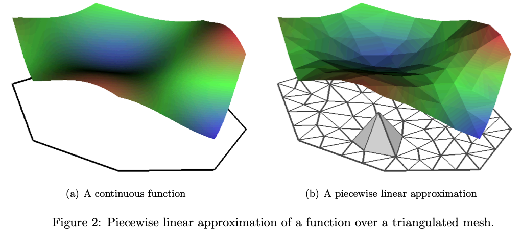
With this fixed, the natural finite element space to use is the space of continuous piecewise linear functions. Traditionally, this is done using combinations of tent functions on a triangular mesh.
With this basis, we can get stability estimates by defining \(v\) and \(v_m\) by \(Lv = f\) and \(L_m v_m = f_m\), from which we get \[ \|R_m v\|_B = \|v_m\|_{V_m} \leq A\|f\|_{L_2} \] which holds, in particular, when the \(L\) has no first order derivatives64.
An oddity about this structure is that functions in \(V_m\) are not not continuously differentiable, while the sample paths of \(u\) almost surely are65. This means that \(V_m\) isn’t necessarily a subset of \(B\) as we would naturally define it. In this case, we need to inflate \(B\) to be big enough to contain the \(V_m\). So instead of taking \(B = C^1(\Omega)\), we need to take \(B = C(\Omega)\) or \(B = L^2(\Omega)\).
This has implications on the smoothness assumptions on \(\Phi(u;y)\), which will need to hold uniformly over \(B\) and \(V_m\) if \(V_m \not \subset B\) and on the set of functionals \(G(u)\) that we use to measure convergence.
A bit of perspective
The critical difference between the SPDE method and the subset-of-regressors approximation is that for the SPDE method, the stability constant \(A_m = A\) is independent of \(m\). This will be important, as this constant pops up somewhere important when we are trying to quantify the error in the finite dimensional approximation.
On the other hand, the SPDE method only works in three and fewer dimensions and while it allows for quite flexible covariance structures66, it is can only directly construct Gaussian processes with integer numbers of continuous derivatives. Is this a problem? The asymptotics say yes, but they only hold if we are working with the exact Gaussian process (or, I guess, if we let the dimension of \(V_m\) hurtle off towards infinity as we get more and more data).
In practice, the Gaussian processes constructed via SPDE methods perform very well on real data67. I suspect part of this is that the stable set of basis functions are very good at approximating functions and the misspecification error plays off against the approximation error.
Bounding the approximation error
With all of this setup, we are finally ready to bound the error between the posterior we would get with the full Gaussian process prior and the posterior we would get using the finite dimensional Gaussian process prior.
We are going to deal with a simpler scenario than the paper we are (sort of) following, because in that situation, I was forced to deal with simultaneously approximating the likelihood and honestly who needs that trouble.
To remind ourselves, we have two priors: the full fat Gaussian process prior, the law of which we denote \(\mu_0\) and the one we could possibly work with \(\mu_0^m\). These lead to two different posteriors \(\mu_y\) and \(\mu_y^m\) given by \[ \frac{d\mu_y}{d\mu_0}(u) = \frac{1}{Z}\mathrm{e}^{-\Phi(u;y)} \quad \text{and}\quad \frac{d\mu_y^m}{d\mu_0^m}(u) = \frac{1}{Z_m}\mathrm{e}^{-\Phi(u;y)} , \] where \(Z_1\) and \(Z_m\) are normalising constants.
We assume that the Gaussian process \(u\) is supported on some Banach space \(V \subseteq B\) and the approximating spaces \(V_m \subset B\). This covers the case where the approximating functions are rougher than the true realisations of the Gaussian process we are approximating. With this notation, we have the restriction operator \(R_m\) that satisfies \[ \|R_mf\|_{V_m} \leq A_m \|f\|_V, \] which is a slightly more targeted bound when \(B\) is larger than \(V\).
We will make the following assumptions about the negative log-likelihood (or potential function) \(\Phi\): For every \(\epsilon > 0\), \(r> 0\), and68 \(\|y\| < r\), there exist positive constants \(C_1, C_2, C_3, C_4\) that may depend on \(\epsilon\) and \(r\) such that the following 4 conditions hold. (Note: when the norm isn’t specified, we want it to hold over both the \(V\) and \(B\) norms.)
For all \(u \in V \cup \left(\bigcup_{m\geq 1} V_m\right)\) \[ \Phi(u;y) \geq C_1 - \epsilon \|u\|^2 \]
For every \(u\in B\), \(y \in Y\) with \(\max \{\|u\|, \|y\|_Y\} < r\), \[ \Phi(u;y) \leq C_2 \]
For every \(\max \{\|u_1\|_V, \|u_2\|_B, \|y\|_Y\} < r\), \[ |\Phi(u_1; y) - \Phi(u_2; y )| \leq \exp\left(\epsilon\max\{\|u_1\|_V^2, \|u_2\|_B^2\} - C_3\right) \|u_1 - u_2\|_B \]
For every \(u\in B\) and \(\max \{\|y_1\|_Y, \|y_2\|_Y\} < r\), \[ |\Phi(u; y_1) - \Phi(u; y_2) | \leq \exp\left(\epsilon \|u\|^2 + C_4\right)\|y_1 - y_2\|_Y \]
These restrictions are pretty light and are basically what are needed to make sure the posteriors exist. The first one say “don’t grow too fast” to the likelihood and is best explained while humming ABBA’s Slipping Through My Fingers. The second one makes sure the likelihood isn’t zero. The third and fourth are Lipschitz conditions that basically make sure that a small change in \(u\) (or \(y\)) doesn’t make a big change in the likelihood. It should be pretty clear that if that could happen, the two posteriors wouldn’t be close.
We are also going to need some conditions on our test functions. Once again, we need them to apply over \(V\) and \(B\) when no space is specified for the norm.
For all \(u \in V\), \(G(u) = \exp(\epsilon \|u\|^2_V+ C_5)\)
For all \(u_1 \in V\), \(u_2 \in V_m\), \[ |G(u_1) - G(u_2)| \leq \exp(\epsilon\max\{\|u_1\|^2_V, \|u_2\|^2_B\})\|u_1 - u_2\|_B. \]
Under these conditions, we get the following theorem, which is a simplified version of Theorem A2 here.
Theorem 1 Under the above assumptions, \[ \left|\mathbb{E}_{\mu_y}(G(u)) - \mathbb{E}_{\mu^m_y}(G(u_m))\right| \leq C_m \sup_{f \in V}\left(\frac{\|f - R_m f\|_B}{\|f\|_V}\right), \] where \(C_m\) only depends on \(m\) through \(A_m\).
I seriously doubt that the dependence on \(A_m\) is exponential, as it is in the proof, but I’m not going to try to track that down. That said, I’m also quite sure that the dependence \(C_m\) is not uniform in \(m\) unless \(A_m\) is constant.
It’s also worth noting that there’s nothing special about \(G\) being real-valued. In general it can take values in any Banach space \(E\). Just replace all those absolute values with norms. That means that the result covers convergence of approximations to things like covariance matrices.
Proof, if you’re interested
We are interested in approximating \[ e_G = \left|\mathbb{E}_{\mu_y}(G(u)) - \mathbb{E}_{\mu^m_y}(G(u_m))\right|. \] We can expand this to get \[\begin{align*} e_G \leq & \frac{1}{Z}\left|\mathbb{E}_{\mu_0}\left(G(u)\exp(-\Phi(u;y))\right) - \mathbb{E}_{\mu_0^m}\left(G(u_m)\exp(-\Phi(u_mm;y))\right)\right| \\ &\quad + \left|\frac{1}{Z} - \frac{1}{Z_m}\right|\mathbb{E}_{\mu_0^m}\left(|G(u_m)|\exp(-\Phi(u_m;y))\right). \\ &= B_1 + B_2. \end{align*}\]
It follows from Andrew Stuart’s work that the normalising constants \(Z\) and \(Z_m\) can be bounded above and below independently of \(m\), so the above expression makes sense.
We will now attack \(B_1\) and \(B_2\) separately. To do this, we need to consider the joint prior \(\lambda_0(u, u_m)\) that is the joint law of the Gaussian process \(u\) and its finite dimensional approximation \(u_m = R_m u\).
For \(B_1\) we basically use the same trick again. \[\begin{align*} ZB_1 \leq & \mathbb{E}_{\lambda_0}\left(|G(u)|\left|\exp(-\Phi(u;y)) -\exp(\Phi(u;y))\right| \right) \\ &\quad + \mathbb{E}_{\lambda_0}\left(\exp(-\Phi(u_m;y)) | G(u) - G(u_m)|\right) \\ &\leq \mathbb{E}_{\lambda_0}\left(\mathrm{e}^{C_5 + \epsilon \|u\|_V^2}\mathrm{e}^{\epsilon\max\{1,A_m\}\|u\|_v^2 - C_1} \mathrm{e}^{\epsilon\max\{1,A_m\}\|u\|_V^2 + C_3}\|u - u_m\|_B\right) \\ & \quad +\mathbb{E}_{\lambda_0}\left(\mathrm{e}^{\epsilon A_m\|u\|_V^2 - C_1}\mathrm{e}^{\epsilon\max\{1,A_m\}\|u\|_V^2 + C_6}\|u - u_m\|_V\right) \\ &\leq \sup_{f \in V}\left(\frac{\|f - R_m f\|_B}{\|f\|_V}\right) \mathrm{e}^{C_3 + C_5 + C_6 -2 C_1}\mathbb{E}_{\mu_0}\left(\|u\|_V\mathrm{e}^{(1+3\max\{1,A_m\} + A_m)\epsilon \|u\|_V^2}\right)\\ &\leq C_7 \sup_{f \in V}\left(\frac{\|f - R_m f\|_B}{\|f\|_V}\right), \end{align*}\] where the second inequality comes from using all of the assumptions on \(\Phi\) and \(G\) and noting that \(\left|e^{-x} - e^{-y}\right| \leq e^{-\min\{x,y\}}|x-y|\); and the final inequality comes from Fernique’s theorem, which implies that expectation is finite.
We can also bound \(B_2\) by noting that \[\begin{align*} \left|Z^{-1} - Z_m^{-1} \right| & \leq \max \{Z^{-2}, Z_m^{-2}\}\mathbb{E}_{\lambda_0}\left(|\exp(-\Phi(u;y)) - \exp(-\Phi(u_m;z))\right) \\ &\leq C_8 \sup_{f \in V}\left(\frac{\|f - R_m f\|_B}{\|f\|_V}\right) \end{align*}\] by the same reasoning as above.Dealing with the approximation error
The theorem above shows that the worst-case error in posterior functionals caused by replacing a Gaussian process \(u\) with it’s approximation \(u_m = R_m u\) is driven entirely by how well a general function from \(V\) can be approximated by a function in \(V_m\). This is not really a surprising result: if the approximation \(u_m\) is unable to approximate the sample paths of \(u\) it is very unlikely it will do a good job with all functionals.
Thankfully, approximation error is one of the better studied things in this world. Especially in the case where \(V = B\).
For instance, it’s pretty easy to show69 that if \(u\) has \(\nu\) derivatives, then \(e_G \leq Cm^{-\frac{\nu}{d} + \epsilon}\) for all \(\epsilon>0\).
If you dive deep enough into the literature, you can get similar results for the type of approximation underneath the subset of regressors approximation.
For the SPDE approximation, it’s all a little bit more tricky as \(V_m \not \subset V\). But ultimately, you get that, for any \(\epsilon >0\), \(e_G \leq C h^{1-\epsilon}\), where \(h\) is a measure of the mesh size70. This is roughly what you’d expect, there’s a loss of \(\epsilon\) from the ordinary interpolation rate which may or may not be a result of me being a bit shit at maths.
The argument that gets us here is really cute so I’ll sketch it below. This is here for two reasons: firstly, because I think it’s cool and secondly because the paper is so compressed it’s hard to completely follow the argument, so I thought it would be nice to put on here. (It also took me a whole afternoon to decipher the proof in the paper, which is usually a sign that it could do with a bit of a re-write. How successfully I clarified it is something I will leave up to others to decide.)
Finite element shit
Setup. Gird yourselves!
We are going to bound that error rate in a way that’s relevant for the finite element method. The natural choices for the function spaces are \(V = H^{1-\epsilon}(\Omega)\) for some fixed \(0 < \epsilon < 1/2\) (close to zero is what we want). and \(B = L^2(\Omega)\). (To be honest the domain \(\Omega\) isn’t changing so I’m gonna forget it sometimes.)
Once again, we’re going to assume that \(L\) is a second order uniformly elliptic PDE with no first-order terms (aka \(b_1 = \cdots = b_d = 0\)) and that \(b_0(s) >0\) on some subset of \(\Omega\). We will use the symmetric, coercive bilinear form associated71 with \(L\), which we can define, for any \(u,v \in H^1\), as \[ a(u, v) = \int_\Omega (A(s)\nabla u(s))\cdot \nabla v(s)\,ds + \int_\Omega b_0(s) u(s)v(s)\,ds \]
Remembering that \(R_m = LL_m^\dagger\), we have \[ \sup_{v \in V}\frac{ \left\|v - R_m v\right\|_B}{\|v\|_V} =\sup_{f\in LV}\frac{ \left\|L^{-1}f - L_n^{\dagger}f\right\|_B}{\|L^{-1}f\|_V}. \]
The set of functions \(f \in LV\) is the set of all functions \(f = Lv\) for some \(v \in V\). It can be shown that \(LV = H^{-1-\epsilon}\), where the negative index indicates a dual Sobolev space (aka the space of continuous linear functionals on \(H^{1+ \epsilon}\)).
This means that we are looking at the difference between the solution to \(Lu = f\) and \(L_m u_m = f_m\), where \(f_m\) is the \(L^2\)-orthogonal projection of \(f\) onto \(V_m\), which is the space of piecewise linear functions on some72 triangular mesh \(\mathcal{T}_m\).
We define the projection of the function \(f \in H^{-1-\epsilon}(\Omega)\) onto \(V_m\) as the unique function \(f_m \in V_m\) such that73 \[ \int_\Omega f_n(s) v_n(s)\,ds = \int f(s) v_n(s)\,ds, \quad \forall v_n \in V_n. \]
Now let’s do this!
With all of this in place, we can actually do something. We want to bound \[ \frac{\|u - u_m\|_{L^2}}{\|u\|_{H^{1+\epsilon}}}, \] where74 \(a(u, \phi) = \int_\Omega f(s) \phi(s)\,ds\) for all \(\phi \in H^{1+\epsilon}\) and \(a(u_m, \phi_m) = \int_\Omega f(s) \phi_m(s)\,ds\) for all \(\phi_m \in V_m \subset H^{1+\epsilon}\).
The key observation is that \[ \int_\Omega f(s) \phi_m(s)\,ds = \int_\Omega f_m(s) \phi_m(s)\,ds, \] which suggests that \(u_m(s)\) is an approximation to two different problems!
Let’s write this second problem down! We want to find \(z^{(m)}\) such that \[ a({z}^{(m)}, \phi) = \int_\Omega f_n(s) \phi(s)\,ds \quad \forall \phi \in H^{1} , \] where the \(m\) superscript indicates that it depends on \(m\) through it’s right hand side. The projection \(f_n \in L^2\), which means that we are in the realm of usual PDEs and (assuming some regularity) \(z^{(m)} \in H^2\).
Hence, we can write \[ \|u - u_m\|_{L^2}\leq \|u - z^{(m)}\|_{L^2} + \|z^{(m)} - u_m\|_{L^2}. \]
We can bound the second term almost immediately from standard finite element theory, which says that \[ \|z^{(m)} - u_m\|_{L^2} \leq Ch^2 \|f_n\|_{L^2}. \]
To estimate \(\|f_m\|\) we use the inverse estimates of Ben Belgacem and Brenner to show that, for any \(v\in L^2(\Omega)\), \[ \int_\Omega f_m(s) v(s) \,ds = \int_\Omega f(s)v_m(s) \,ds\leq\|f\|_{H^{-1-\epsilon}}\|v_m\|_{H^{1+\epsilon}} \leq Ch^{-1-\epsilon} \|f\|_{H^{-1-\epsilon}} \|v\|_{L^2}, \] where \(v_m\) is the orthogonal projection of \(v\) onto \(V_m\).
If we set \(v = f_m\) in the above equation, we get \(\|f_m\|_{L^2} \leq Ch^{-1-\epsilon} \|f\|_{H^{-1-\epsilon}}\), which combines with our previous estimate to give \[ \|z^{(m)} - u_m\|_{L^2} \leq Ch^{1-\epsilon} \|f_n\|_{L^2}. \]
Finally, to bound \(\|u - z^{(m)}\|_{L^2}\) we are going to use one of my75 favourite arguments. Fix \(w \in L^2\) and let \(W\) be the solution of the dual equation \(a(\phi, W) = \int_\Omega \phi(s)w(s)\,ds\). It then follows that, for any \(v_m \in V_m\), \[\begin{align*} \left|\int_\Omega (u(s) - z^{(m)}(s))w(s)\,ds\right| &= \left|a(u - z^{(m)}, W)\right| \\ &= \left|\int_\Omega (f(s) - f_m(s))W(s)\,ds\right|\\ &= \left|\int_\Omega (f(s) - f_m(s))(W(s) - v_m(s))\,ds\right|\\ &\leq\left|\int_\Omega f(s)(W(s) - v_m(s))\,ds\right|+ \left|\int_\Omega f_m(s)(W(s) - v_m(s))\,ds\right| \\ &\leq \|f\|_{H^{-1-\epsilon}}\|W - v_m\|_{H^{1+\epsilon}} + Ch^{-1-\epsilon} \|f\|_{H^{-1-\epsilon}} \|W - v_m\|_{L^2} \\ &\leq C \|f\|_{H^{-1-\epsilon}} h^{-1 -\epsilon}\left(h^{1+\epsilon}\|W - v_m\|_{H^{1+\epsilon}} + \|W - v_m\|_{L^2} \right), \end{align*}\] where the first line uses the definition of \(W\); the second uses the definition of \(u\) and \(z^{(m)}\); the third uses the fact that \((f - f_m) \perp V_m\) so subtracting off \(v_m\) doesn’t change anything; the fourth is the triangle inequality; the fifth is the Hölder inequality on the left and the estimate from half a screen up on the right; and the sixth line is clean up.
Because the above bound holds for any \(v_m \in V_m\), we can choose the one that makes the bound the smallest. This leads to \[\begin{align*} \left|\int_\Omega (u(s) - z^{(m)}(s))w(s)\,ds\right| &\leq C \|f\|_{H^{-1-\epsilon}} h^{-1 -\epsilon}\inf_{v \in V_m}\left(h^{1+\epsilon}\|W - v_m\|_{H^{1+\epsilon}} + \|W - v_m\|_{L^2} \right) \\ & \leq C\|f\|_{H^{-1-\epsilon}} h^{-1 -\epsilon} h^2 \|W\|_{H^2}\\ &\leq C h^{1-\epsilon} \|w\|_{L^2}, \end{align*}\] where the last two inequalities are Theorem 14.4.2 from Brenner and Scott and a standard estimate of the solution to an elliptic PDE by it’s RHS.
Putting this all together we get the result. Phew.
This whole argument was a journey, but I think it’s quite pretty. It’s clobbered together from a lot of sleepless nights and an argument inspired by strip-mining76 a Ridgeway Scott paper from 1976. Anyway, I think it’s nifty.
Wrapping it up
So. That was quite a lot. I enjoyed it, but I’m weird like that. This has mostly been me trying to remember what I did in 2015. Why? Because I felt like it.
I also think that there’s some value in this way of thinking about Gaussian processes and it’s nice to show off some ways to use all of that weird shit in the last post.
All of these words can be boiled down to this take away:
If your finite dimensional GP \(u_m\) is linked to a GP \(u\) by some (potentially non-linear relationship) \(u_m= R_m u\), then the posterior error will be controlled by how well you can approximate a function \(v\) that could be a realisation of the GP by \(R_m v\).
This is a very intuitive result if you are already thinking of GP approximation as approximating a random function. But a lot of the literature takes a view that we are approximating a covariance matrix or a multivariate normal. This might be enough to approximate a maximum likelihood estimator, but it’s insufficient for approximating a posterior77
Furthermore, because most of the constants in the bounds don’t depend too heavily on the specific finite dimensional approximation (except through \(A_m\)), we can roughly say that if we have two methods for approximating a GP, the one that does a better job at approximating functions will be the better choice.
As long as it was, this isn’t a complete discussion of the problem. We have not considered hyper-parameters! This is a little bit tricky because if \(\mu_0\) depends on parameters \(\theta\), then \(R_m\) will also depend on parameters (and for subset of regressors, \(V_m\) also depends on the parameters).
In theory, we could use this to bound the error in the posterior \(p(\theta \mid y)\). To see how we would do that, let’s consider the case where we have Gaussian observations.
Then we get \[\begin{align*} p(\theta \mid y) & \frac{\exp(-\Phi(u;y))}{p(y)} \left[\frac{d\mu_y}{d\mu_0}\right]^{-1} p(\theta) \\ &= \frac{Z(\theta) p(\theta)}{\int_\Theta Z(\theta)p(\theta)\,d\theta}, \end{align*}\] where \(Z(\theta) = \mathbb{E}_{\mu_0}\left(e^{-\Phi(u;y)}\right)\).
We could undoubtedly bound the error in this using similar techniques to the ones we’ve already covered (in fact, we’ve already got a bound on \(|Z - Z_m|\)). And then it would just be a matter of piecing it all together.
Footnotes
Naively: a condescending way to say “the way you were told to use them”↩︎
Is it better to have a large amount of crappy data or a small amount of decent data? Depends on if you’re trying to impress people by being right or by being flashy.↩︎
Who doesn’t love a good shape. Or my personal favourite: a point pattern.↩︎
Or, hell, this is our information about how to query the Gaussian process to get the information we need for this observation. Because, again, this does not have to be as simple as evaluating the function at a point!↩︎
This could be time, space, space-time, covariate space, a function space, a lattice, a graph, an orthogonal frame, a manifold, a perversion, whatever. It doesn’t matter. It’s all just Gaussian processes. Don’t let people try to tell you this shit is fancy.↩︎
This could be covariate information, group information, hierarchy information, causal information, survey information, or really anything else you want it to be. Take a deep breath. Locate your inner peace. Add whatever you need to the model to make it go boop.↩︎
I will never use this assumption. Think of it like the probability space at the top of a annals of stats paper.↩︎
So the thing is that this is here because it was funny to me when I wrote it, but real talk: just being like “it’s iid” is some real optimism (optimism, like hope, has no place in statistics.) and pretending that this is a light or inconsequential assumption is putting some bad energy out into the world. But that said, I was once a bit drunk at a bar with a subjective Bayesian (if you want to pick your drinking Bayesian, that’s not a bad choice. They’re all from The North) and he was screaming at me for thinking about what would happen if I had more data, and I was asking him quietly and politely how the data could possibly inform models as complex as he seemed to be proposing. And he said to me: what you do is you look for structures within your data that are exchangeable in some sense (probably after conditioning) and you use those as weak replicates. And, of course, I knew that but I’d never thought about it that way. Modelling, eh. Do it properly.↩︎
These (and the associated parenthetical girls) were supposed to be nested footnotes but Markdown is homophobic and doesn’t allow them. I am being oppressed.↩︎
It’s an interesting area, but the tooling isn’t there for people who don’t want to devote a year of their lives to this to experiment.↩︎
This is what matrix nerds say when they mean “I love you”. Or when they mean that it’s all derived from the structure of a matrix rather than from some structural principles stolen from the underlying problem. The matrix people are complicated.↩︎
The reason for this is that, while there are clever methods for getting determinants of H-matrices, they don’t actually scale all that well. So Geoga, Anitescu, and Stein paper use a Hutchinson estimator of the log-determinant. This has ok relative accuracy, but unfortunately, we need it to have excellent absolute accuracy to use it in a Bayesian procedure (believe me, I have tried). On the other hand, the Hutchinson estimator of the gradient of the log-determinant is pretty stable and gives a really nice approximate gradient. This is why MLE type methods for learning the hyper-parameters of a GP can be made scalable with H-matrix techniques.↩︎
Otherwise, why bother. Just sub-sample and get on the beers. Or the bears. Or both. Whatever floats your boat.↩︎
on \(u\) and probably other parameters in the model↩︎
Dual spaces, y’all. This vector was inevitable because \(m\)-dimensional row vectors are the dual space of \(\mathbb{R}^m\), while \(s_i \rightarrow u(s_i)\) is in \(B^*\).↩︎
This is not surprising if you’re familiar with the sketching-type bounds that Yang, Pilanci and Wainwright did a while back (or, for that matter, with any non-asymptotic bounds involving the the complexity of the RKHS). Isn’t maths fun.↩︎
Hölder↩︎
Think “infinitely differentiable but more so”.↩︎
An analytic function is one that you know will walk straight home from the pub, whereas a \(\nu\)-differentiable function might just go around the corner, hop on grindr, and get in a uber. Like he’s not going to go to the other side of the city, but he might pop over to a nearby suburb. A generalised function texts you a photo of a doorway covered by a bin bag with a conveniently placed hole at 2am with no accompanying message other than an address↩︎
I mean, I cannot be sure, but I’m pretty sure.↩︎
Again, not strictly necessary but it removes a tranche of really annoying technicalities and isn’t an enormous restriction in practice.↩︎
The result is that there is no non-trivial translation invariant measure on a separable Banach space (aka there is no analogue of the Lebesgue measure). You can prove this by using separability to make a disjoint cover of equally sized balls, realise that they would all have to have the same measure, and then say “Fuck. I’ve got too many balls”.↩︎
Borel. Because we have assumed \(B\) is separable, the cylindrical \(\sigma\)-algebra is identical to the Borel \(\sigma\)-algebra and \(\mu_0\) is a Radon measure. Party.↩︎
See Andrew Stuart’s long article on formulating Bayesian problems in this context and Masoumeh Dashti and Andrew Stuart’s paper paper on (simple) finite dimensional approximations.↩︎
The SPDE approach. Read on Macduff.↩︎
This covers GP models, GAMs, lots of spatial models, and a bunch of other stuff.↩︎
Like, the data is a single observation of a point pattern. Or, to put it a different way, a list of (x,y) coordinates of (a priori) unknown length.↩︎
Approximate Markovian GPs in 2-4 dimensions. See here for some info↩︎
Rue. The king of INLA. Another all round fabulous person. And a person foolish enough to hire me twice even though I was very very useless.↩︎
In the interest of accuracy, Janine and I were giving back to back talks at a conference that we decided for some reason to give as a joint talk and I remember her getting more and more agitated as I was sitting in the back row of the conference desperately trying to contort the innards of INLA to the form I needed to make the damn thing work. It worked and we had results to present. We also used the INLA software in any number of ways it had not been used before that conference. The talk was pretty well received and I was very relieved. It was also my first real data analysis and I didn’t know to do things like “look at the data” to check assumptions, so it was a bit of a clusterfuck and again Janine was very patient. I was a very useless 25 year old and a truly shit statistician. But we get better if we practice and now I’m a perfectly ok statistician.↩︎
Janine and I, with Finn Lindgren, Sigrunn Sørbye and Håvard Rue, who were all heavily involved throughout but I’m sure I’ve already exhausted people’s patience.↩︎
IIRC, Sigrunn’s university has one of those stupid lists where venue matters more than quality. Australia is also obsessed with this. It’s dumb.↩︎
In hindsight, the reviewer was asking for a simulation study, which is a perfectly reasonable thing to ask for but at the time I couldn’t work out how to do that because, in my naive numerical analyst ways, I thought we would need to compare our answer to a ground truth and I didn’t know how to do that. Now I know that the statistician way is to compute the same thing two different ways on exactly one problem that’s chosen pretty carefully and saying “it looks similar”.↩︎
Conditional on the log-intensity surface, a LGCP is a Poisson process↩︎
is it, though↩︎
My co-authors are all very patient.↩︎
with fixed hyper-parameters↩︎
The thing about inverse problems is that they assume \(\Phi(u;y)\) is the solution of some PDE or integral equation, so they don’t make any convenient simplifying assumptions that make their results inapplicable to LGCPs!↩︎
https://arxiv.org/pdf/0901.1342.pdf↩︎
star↩︎
Also weak convergence but metrized by the Wasserstein-1 distance.↩︎
Fernique’s Theorem. I am using “we” very liberally here. Fernique knew and said so in French a while back. Probably the Soviet probabilists knew too but, like, I’m not going to write a history of exponential moments.↩︎
On \(L^2\), which is a Hilbert space so the basis really is countable. The result is a shit-tonne easier to parse if we make \(B\) a separable Hilbert space but I’m feeling perverse. If you want the most gloriously psychotic expression of this theorem, check out Theorem 7.3 here↩︎
There are tonnes of examples where people do actually use the Karhunen-Loève basis or some other orthogonal basis expansion. Obviously all of this theory holds over there.↩︎
This has many names throughout the literature. I cannae be arsed listing them. But Quiñonero-Candela, Rasmussen, and Williams attribute it to Wahba’s book in 1990.↩︎
Functions of the form \(\sum_{i=1}^m a_j r_u(\cdot, s_j)\) are in the RKHS corresponding to covariance function \(r_u\). In fact, you can characterise the whole space as limits of sums that look like that.↩︎
I mean, we are not going to be using the \(A_m\) to do anything except grow with \(m\), so the specifics aren’t super important. Because this is a blog post.↩︎
Not every. You do this for nice sets. See Rozanov’s book on Markov random fields if you care.↩︎
\(d(s, A) = \inf_{s'\in A} \|s - s'\|\)↩︎
Rozanov↩︎
The sets on which they are non-zero are different↩︎
For general Markov random fields, this representation still exists, but \(L\) is no longer a differential operator (although \(L^*L\) must be!). All of the stuff below follows, probably with some amount of hard work to get the theory right.↩︎
What is white noise? It is emphatically not a stochastic process that has the delta function as it’s covariance function. That thing is just ugly. In order to make any of this work, we need to be able to integrate deterministic functions with respect to white noise. Hence, we view it as an independently scattered random measure that satisfies \(W(A) \sim N(0, |A|)\) and \(\int_A f(s)W(ds) \sim N(0, \int_A f(s)^2\, ds)\). Section 5.2 of Adler and Taylor’s book Random Fields and Geometry is one place to learn more.↩︎
Finite element methods had been used before, especially in the splines community, with people like Tim Ramsay doing some interesting work. The key insight of Finn’s paper was to link this all to corresponding infinite dimensional Gaussian processes.↩︎
We’re assuming \(V_m\subset L^2(\Omega)\), which is not a big deal.↩︎
See the paper for details of exactly which pseudo-inverse. It doesn’t really matter tbh, it’s just we’ve got to do something with the other degrees of freedom.↩︎
Consult your favourite finite element book and then get pissed off it doesn’t cover higher-order PDEs in any detail.↩︎
It looks like this is vital, but it isn’t. The main thing that changes if your PDE is hyperbolic or parabolic or hypo-elliptic is how you do the discretisation. As long as the PDE is linear, this whole thing works in principle.↩︎
For some \(\alpha>0\), \(\sum_{i,j=1}^d w_iw_ja_{ij}(s) \geq \alpha \sum_{i=1}^d w_i^2\) holds for all \(s \in \Omega\).↩︎
For this construction to work in higher dimensions, you need to use a higher-order differential operator. In particular, if you want a continuous field on some subset of \(\mathbb{R}^d\), you need \(L\) to be a differential operator of order \(>d/2\) or higher. So in 4 dimensions, we need the highest order derivative to be at least 4th order (technically \(L\) could be the square root of a 6th order operator, but that gets hairy).↩︎
It holds in general, but if the linear terms are dominant (a so-called advection-driven diffusion), then you will need a different numerical method to get a stable estimate.↩︎
Modulo some smoothness requirements on \(\Omega\) and \(a_{ij}(s)\).↩︎
It’s very easy to model weird anisotropies and to work on manifolds↩︎
Let’s not let any of the data fly off to infinity!↩︎
Corollary A2 in the paper we’re following↩︎
Think of it as the triangle diameter if you want.↩︎
Integration by parts gives us \(\int_\Omega (Lu(s))v(s)\,ds = a(u,v)\) if everything is smooth enough. We do this to confuse people and because it makes all of the maths work.↩︎
not weird↩︎
\(f\) is a generalised function so we are interpreting the integrals as duality pairings. This makes sense because \(V_m \subset H^{1+\epsilon}\) if we allow for a mesh-dependent embedding constant (this is why we don’t use \(B = H^{1+\epsilon}\))↩︎
This is how fancy people define solutions to PDEs. We’re fancy.↩︎
Also everyone else’s, but it’s so elegantly deployed here. This is what I stole from Scott 1976)↩︎
Real talk. I can sorta see where this argument is in the Scott paper, but I must’ve been really in the pocket when I wrote this because phew it is not an obvious transposition.↩︎
Unless the approximation is very, very good. If we want to be pedantic, we’re approximating everything by floating point arithmetic. But we’re usually doing a good job.↩︎
Reuse
Citation
@online{simpson2021,
  author = {Simpson, Dan},
  title = {Getting into the Subspace; or What Happens When You
    Approximate a {Gaussian} Process},
  date = {2021-11-24},
  url = {https://dansblog.netlify.app/getting-into-the-subspace},
  langid = {en}
}